Resistances in Parallel

Resistances in parallel is a common term used in industrial, commercial, and institutional power systems. Therefore, a good understanding of working with resistors in parallel and calculating their various parameters is crucial for maintaining safe and efficient operations.

It means that when resistors are connected in parallel, they share the same voltage across them. Hence, this means that the resistances are in parallel. This is because the total resistance of the resistors in parallel is less than that of any individual resistor, making it a useful configuration for reducing resistance and increasing current in a circuit.

Adding more resistors in parallel reduces the circuit's total resistance, increasing the current. However, adding too many resistors in parallel can overload the circuit and cause it to fail.

Understanding Resistances in Parallel

They refer to the configuration in which two or more resistors are connected side by side across the same voltage points in an electrical circuit. In this arrangement, the voltage across each resistor is the same, while the current is divided among the resistors according to their resistance values. This configuration is commonly used in circuit analysis to simplify complex circuits and determine the equivalent parallel resistance.

Calculating the Equivalent Resistance

To calculate the equivalent resistance of resistances in parallel, the reciprocal of the equivalent resistance (1/Req) is equal to the sum of the reciprocals of the individual resistances (1/R1 + 1/R2 + ... + 1/Rn). This formula is crucial in resistance calculation and helps engineers design efficient power systems that meet the desired voltage drop and current distribution requirements.

To calculate the total resistance of resistors in parallel, the reciprocal of each resistor is added together, and then the result is inverted to give the total resistance. This can be represented mathematically as:

1/Rt = 1/R1 + 1/R2 + 1/R3 + ...

where Rt is the total resistance and R1, R2, R3, etc. are the individual resistors.

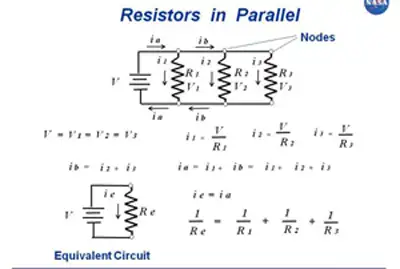
Five resistors R(1) through R(5), connected in parallel, produce a net resistance R.

In a circuit with resistors in parallel, the current is divided among the resistors according to their individual resistance values. This is known as the current division, and it can be calculated using Ohm's law and the circuit's total resistance. The formula for calculating the current through each resistor in parallel is:

I1 = (V/R1) * (R2/(R2 + R3)) I2 = (V/R2) * (R1/(R1 + R3)) I3 = (V/R3) * (R1/(R1 + R2))

where I1, I2, and I3 are the currents through each resistor, V is the voltage across the circuit, and R1, R2, and R3 are the individual resistors.

Simplifying a circuit with resistors in parallel involves finding the equivalent resistance of the circuit. This is the resistance value that would produce the same current as the original parallel circuit, and it can be calculated using the reciprocal formula:

1/Req = 1/R1 + 1/R2 + 1/R3 + ...

where Req is the equivalent resistance.

Impact on Total Resistance

In a parallel configuration, adding more resistors decreases the total resistance. The reason is that the current has multiple paths to flow through, reducing the overall opposition to current flow. This characteristic is particularly useful in designing power supply systems, where lower resistance is desired to minimize energy losses and improve system efficiency.

Practical Applications

They are employed in various real-life circuits and power systems. For instance, they are commonly found in circuit simulations, power distribution systems, and load balancing applications. In industrial settings, a parallel resistor calculator is often used to measure multiple current paths for fault protection and redundancy. In commercial and institutional power systems, parallel configurations are employed to manage load distribution and ensure system reliability.

Differences between Parallel and Series Connections

In a series circuit, resistors are connected end-to-end, and the current flows consecutively from the source of each resistor. The total resistance in a series circuit equals the sum of individual resistances, and the voltage drop across each single resistor is different. In contrast, they share the same voltage, and the total resistance decreases as more resistors are added. Identifying these connections in a circuit diagram is crucial for proper circuit analysis and design.

Combining Resistances in Parallel and Series

They can be combined with resistances in series within the same circuit. In such cases, equivalent resistances for both parallel and series sections are calculated separately. Then, the total resistance is determined by adding the equivalent resistances of the series and parallel sections. This approach helps engineers analyze complex circuits and design efficient power systems.

They are crucial to industrial, commercial, and institutional power systems. Understanding how to calculate the total resistance, current distribution, and power dissipation of resistors in parallel is essential for maintaining safe and efficient operations. In addition, engineers can optimize their designs for optimal performance by using circuit simulation software and other tools.