Active Power

Electricity prices reflect tariffs, kWh rates, time-of-use schedules, peak demand charges, and grid congestion, driven by generation costs, transmission losses, and load profiles in power systems and industrial electrical engineering.

What Are Electricity Prices?

Electricity prices are costs per kWh shaped by tariffs, time-of-use, demand charges, and grid operating constraints.

✅ Defined per kWh with time-of-use and demand charges

✅ Influenced by generation mix, transmission losses, congestion

✅ Managed via load control, demand response, smart metering

Electricity prices, or rates, are usually determined by electric utilities and the governmental organizations that oversee them. The fees an electric utility company charges its customers for service aer based on electricity prices set by government, except in the case where they cost electricity prices on a deregulated basis. In that case, electricity prices are determined by marketplace factors such as supply and demand. Electric utility companies charge their customers different rates, depending on the type of customer, the kind of contract, and on the customer's needs. Electricity Prices bill energy on the kwh basis of the individual customer's rate, the level of consumption, and other charges, such as taxes and fuel adjustments. This is how electricity billed. For a deeper breakdown of typical rate components, resources like electricity cost guides explain line items and surcharges clearly.

That collection of rates is called a tariff. The power tariff is designed to provide the privately owned electric utility with enough income to allow investors to earn a cash return and cover operation and maintenance costs. Most of the larger utilities operate as regulated franchises, meaning that the prices they charge are subject to public review, often by a State public utility commission. In competitive markets, customers may choose an electricity supplier while the utility still handles delivery services and billing oversight.

Publicly owned electric utilities are nonprofit, local government agencies established to provide service to their communities and nearby consumers at cost, returning excess funds to the consumer in the form of community contributions, more economic and efficient facilities, and lower power rates. To meet these community objectives, public power agencies plan their electricity supply over multiyear horizons to manage risk and affordability.

Publicly owned electric utilities (which number approximately 2,000) include municipals, public power districts, State authorities, irrigation districts, and other State organizations. Some of these organizations also own or contract for electricity generation assets to enhance self-sufficiency and rate stability.

There are approximately 900 cooperative electric utilities in the United States currently doing business in 47 States. These utilities are owned by their members and are established to provide power to those members. Because member education supports better usage decisions, many cooperatives provide primers on what electricity is and how it is measured on bills.

Average retail Electricity prices of power are calculated by dividing utility revenue by retail sales. The resulting measurement is the cost, or average revenue per kilowatthour, of power sold. (A kilowatthour is equal to one watt of power supplied to an electric circuit steadily for 1,000 hours.) Electric utilities usually offer three primary classes of service: residential, commercial, and industrial. The average price per kilowatthour for residential consumers is generally higher than for any other sector due in part to higher costs associated with serving many consumers who use relatively small amounts of power. In Ontario, the industrial sector has the lowest energy prices and energy bills rates every month due to the economies of serving a few consumers who use relatively large amounts of electricity. Understanding the distinction between energy in kilowatthours and instantaneous electricity power demand helps customers interpret peak charges and capacity fees. Regional consumption patterns, including trends in electricity demand in Canada, can influence wholesale prices and cross-border power flows affecting local rates.

Related Articles

• Electricity Fundamentals

• Electricity Questions

• Electricity History

Active power is the actual energy consumed by electrical equipment to perform useful work, such as lighting or running motors. It is measured in kilowatts (kW) and is essential for efficient power system design, load management, and energy billing accuracy.

What is "active power"?

Active power is the real power consumed in an AC circuit to perform useful work.

✅ Measured in kilowatts (kW)

✅ Powers resistive loads like heaters, lights, and motors

✅ Crucial for calculating energy usage and efficiency

In AC circuits, active power (P) refers to the component of electrical power that results in energy transfer to a load. It is the energy that performs work—such as producing motion, light, or heat—and is distinct from reactive power, which oscillates between source and load without being consumed.

Active Power Formula

The general formula for active power is:

P = VIcosθ

Where:

• P = Active Power (watts)

• V = RMS Voltage

• I = RMS Current

• θ = Phase angle between voltage and current

In real-world power systems, only the portion of the current in phase with the voltage contributes to active power. The portion out of phase results in reactive power and does not produce usable energy.

Equation 1

The above active power equation is valid for both sinusoidal and nonsinusoidal conditions. For sinusoidal condition, '1rn, resolves to the familiar form,

Equation 2

Sinusoidal and Non-Sinusoidal Conditions

The calculation of active power can differ slightly depending on waveform distortion:

• For sinusoidal conditions, Equation 1 simplifies to the standard P = VIcosθ form.

• For non-sinusoidal waveforms, the total active power includes the sum of contributions from all harmonic components. However, since voltage distortion is typically below 5% in most power systems, the simplified equation is usually accurate enough for practical purposes.

Real-World Example

A standard incandescent light bulb converts electrical power into visible light and heat. This is a classic case of active power at work—where the current and voltage are in phase, and virtually all supplied power is consumed usefully.

Active vs Reactive vs Apparent Power

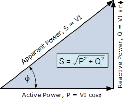
It’s important to distinguish active power from related concepts:

• Reactive Power (Q): Energy exchanged but not consumed, measured in kVAR.

• Apparent Power (S): The vector sum of active and reactive power, measured in kVA.

• Power Factor: The ratio of active power to apparent power (PF = P/S).

While active power does the real work, apparent power impacts system loading and reactive power affects voltage stability. See our power factor training for more.

Measurement and Application

Active power is typically measured using true RMS meters that calculate the average of the instantaneous product of voltage and current. Advanced power analyzers now offer direct measurement of real power in both clean and distorted systems.

Engineers use active power data for:

• Energy consumption analysis

• Load management and optimization

• System efficiency evaluation

• Compliance with energy standards

Related Reading

• Understand the difference between active and reactive power

• Learn how to improve system performance with our power quality analysis training

• Discover how electrical resistance affects power consumption

• Explore the role of power factor correction in reducing energy waste

Frequently Asked Questions

What is active power used for?

Active power is used to perform real work in electrical systems, such as lighting, heating, and running motors.

Is active power the same as real power?

Yes. Active power, real power, and true power are interchangeable terms that refer to the same concept.

How is active power calculated?

It is calculated using the formula P = VIcosθ, where V and I are RMS voltage and current, and θ is the phase angle between them.

In summary, understanding active power is essential for designing efficient electrical systems and ensuring energy accountability. By distinguishing it from reactive and apparent power, professionals can improve system performance and reduce energy losses.

Related Articles

• Electricity Fundamentals

• Electricity Questions

• Electricity History

Alternative electricity integrates renewable energy, smart grids, and distributed generation, combining solar photovoltaics, wind power, hydropower, and battery storage with power electronics and demand response to decarbonize grids and improve reliability.

What Is Alternative Electricity?

Alternative electricity uses renewables, storage, and smart grids to deliver reliable, low-carbon power.

✅ Power electronics enable PV, wind, and storage grid integration

✅ Smart inverters support voltage, frequency, and reactive power control

✅ Microgrids improve resilience with islanding and load management

Alternative electricity power is essential if we are to find affordable and workable sources of energy before the world completely consumes its limited supply of energy sources. Many countries have started to introduce renewable energy schemes and many countries have invested money into researching and even producing different sources of electricity energy. While it is essential that we become less reliant or not reliant at all on fossil fuels, many forms of alternate energy have their disadvantages as well as their obvious advantages. The advantages of alternate energy far outweigh the disadvantages. For a primer on how modern grids convert primary energy into usable power, see this overview of how electricity is generated across different technologies today.

Wind Energy

Harnessing the power of the wind and using it to our ends is hardly a new idea. Windmills have been and still are used for many different purposes and have been for a great many years, but the improvement of turbines combined with the improved technology to turn the motion of turbine blades into an energy source has seen a marked increase in the use of electricity generating turbines. Detailed diagrams explain how turbine blades capture kinetic energy to generate electricity efficiently under varying wind speeds.

Wind power is very popular, but in order to provide a reasonable amount of power it may prove necessary to have large amounts of turbines. On windy days, and even not so windy days some turbines make a noise that many residents consider to be unbearable. Areas of open countryside are protected by conservation orders, which means they can’t be built there either and if there is no conservation order there are still protestors willing to do almost anything to stop the turbines being built. The only viable option left is to use offshore wind farms and these are being investigated, developed and planned all around the world but it takes too many turbines to create a reasonable amount of power and eventually they will have to be built inland; a matter that will be contested wherever the wind farms are proposed to be built.

Understanding capacity factors and grid integration is key to planning electricity production that balances reliability and community impacts.

Wind power is produced by converting wind energy into electricity. Electricity generation from wind has increased significantly in the United States since 1970. Wind power provided almost 5% of U.S. electricity generation in 2015. These trends mirror broader shifts in electricity generation portfolios as states pursue renewable portfolio standards.

Solar Energy

Solar energy is probably the most common form of alternate energy for everyday people and you can see solar lights ad other solar accessories in many gardens. Governments are beginning to offer grants to assist in paying for photovoltaic roof tiles; these tiles are easily fitted onto your roof and collect the heat from the sun. This heat can either be used to heat water or can even be converted into energy electric power. The advantage for the consumer is that by including a grid tie system you can actually sell unused energy back to the grid. Photovoltaic tiles take the place of ordinary roof tiles and can be perfectly blended to fit the look of the outside of your house. With solar energy you too can help the environment.

Many utilities now offer tariffs that credit exports from rooftop systems, linking household budgets to green electricity choices in a transparent way.

Solar power is derived from energy from the sun. Photovoltaic (PV) and solar-thermal electric are the two main types of technologies used to convert solar energy to electricity. PV conversion produces electricity directly from sunlight in a photovoltaic (solar) cell. Solar-thermal electric generators concentrate solar energy to heat a fluid and produce steam to drive turbines. In 2015, nearly 1% of U.S. electricity generation came from solar power. PV and solar-thermal now sit alongside other major sources of electricity in utility planning models.

Biomass

Ask most people which renewable energy source is the most widely used and they would say either wind or solar, but they’d be wrong or at least they certainly would in America. Since 2000 Biomass has been the most highly produced alternate energy in the United States. Using plant and animal material to create energy isn’t without its downfalls. It would almost certainly meet with competition from residents if biomass power stations were to be created in built up areas. The decomposing plants and animal waste creates an awful smell that is incredibly difficult to mask but it is very renewable (there’s always plants and animal waste).

Biomass is material derived from plants or animals and includes lumber and paper mill wastes, food scraps, grass, leaves, paper, and wood in municipal solid waste (garbage). Biomass is also derived from forestry and agricultural residues such as wood chips, corn cobs, and wheat straw. These materials can be burned directly in steam-electric power plants, or they can be converted to a gas that can be burned in steam generators, gas turbines, or internal combustion engine-generators. Biomass accounted for about 2% of the electricity generated in the United States in 2015.

Other renewable energy sources

These are the main three renewable energy sources that the countries of the world are creating at the moment but there are others. Whether nuclear power is a viable alternate or not is a debate that will undoubtedly rage on forever, but it is a renewable energy and some countries already have extensive capabilities to produce it. Modern technology means that nuclear power stations are safer than they’ve ever been and damage to people, animals or plantation is highly unlikely. However, it takes a long time to develop nuclear power station and even plants that are already being built may take ten years to come to fruition.

Renewable energy sources provide 13% of U.S. electricity

Hydropower, the source of about 6% of U.S. electricity generation in 2015, is a process in which flowing water is used to spin a turbine connected to a generator. Most hydropower is produced at large facilities built by the federal government, like the Grand Coulee Dam. The West has many of the largest hydroelectric dams, but there are many hydropower facilities operating all around the country. For a deeper look at how turbines and dams convert flow into water electricity, engineers often study case histories from multiple river systems.

Hydro power is used in some countries and uses the motion of waves to create energy. While it is a possibility, the amount of energy produced is minimal and the outlay to set these schemes up is quite large. Without further investigation and improvement in the techniques used it is unlikely that Hydropower will become a major player in the renewable energy world.

Geothermal power comes from heat energy buried beneath the surface of the earth. In some areas of the United States, enough heat rises close enough to the surface of the earth to heat underground water into steam, which can be tapped for use at steam-turbine plants. Geothermal power generated less than 1% of the electricity in the United States in 2015.

Related Articles

• Electricity Fundamentals

• Electricity Questions

• Electricity History

Capacitors in series lower the total capacitance but increase voltage handling. This configuration is widely used in electronics, circuit design, and energy storage to balance voltage and improve reliability.

What are Capacitors in Series?

Capacitors in series describe a circuit configuration where capacitors are connected end to end, affecting capacitance and voltage distribution.

✅ The total capacitance is always less than the smallest capacitor value

✅ Voltage divides across each capacitor based on its capacitance

✅ Improves voltage rating of circuits while lowering equivalent capacitance

They play a critical role in various electronic applications, and understanding their characteristics, advantages, and potential drawbacks is essential for designing and implementing successful circuits. By mastering the concepts of capacitance, voltage distribution, and energy storage, one can leverage capacitors in series to create optimal circuit designs. To fully understand how capacitors (caps) behave in different setups, it helps to compare Capacitance in Parallel with series connections and see how each affects circuit performance.

Capacitors are fundamental components in electronic circuits, and their applications are vast, ranging from simple timing circuits to sophisticated filtering applications. This article delves into the intricacies of caps connected in series, highlighting their characteristics, advantages, and potential drawbacks.

To understand capacitors in series, it's essential first to grasp the concept of capacitance, which represents a capacitor's ability to store electric charge. Caps consist of two conductive plates separated by a dielectric material that can store energy when an applied voltage is present. The amount of energy stored depends on the capacitance value, voltage rating, and the dielectric material used. Engineers often study Capacitance and its capacitance definition to calculate charge storage and predict how components will interact in series circuits. 

When caps are connected in series, their individual capacitance values contribute to the total equivalent capacitance. The series connection is achieved when the positive plate of one capacitor is connected to the negative plate of the subsequent capacitor. This forms a continuous path for current flow, creating a series circuit.

Calculating the total capacitance for capacitors in series is different from parallel capacitors. In a series connection, the reciprocal of the total equivalent capacitance is equal to the sum of the reciprocals of the individual capacitance values. Mathematically, this is represented as:

1/C_total = 1/C1 + 1/C2 + 1/C3 + ... + 1/Cn

Where C_total is the total equivalent capacitance, and C1, C2, C3, ... Cn are the individual capacitance values of the number of caps connected in series.

In a series connection, the electric charge stored in each capacitor is the same. However, the voltage across each capacitor varies depending on its capacitance. According to Kirchhoff's voltage law, the sum of voltages across individual capacitors must equal the applied voltage. Thus, higher capacitance values will have lower voltage drops, while lower capacitance values will have higher voltage drops.

There are both advantages and disadvantages to connecting capacitors in series. On the plus side, the voltage rating of the series connection increases, allowing the circuit to handle higher voltage levels without risking damage to the caps. This feature is particularly useful in high-voltage capacitors in series applications. Alongside capacitors, Amperes Law and Biot Savart Law provide deeper insight into the electromagnetic principles that govern current and voltage distribution.

However, there are also drawbacks to this arrangement. The total equivalent capacitance decreases as more capacitors are added to the series, which may limit the energy storage capabilities of the circuit. Moreover, in the event of a capacitor failure, the entire series connection is compromised.

Different capacitor types and values can be combined in a series configuration, but care must be taken to consider each capacitor's voltage ratings and tolerances. For instance, mixing capacitors with different dielectric materials may lead to uneven voltage distribution and reduced overall performance. Since Capacitors are essential to energy storage and timing circuits, learning their behavior in a Capacitors in Series arrangement is key for advanced electronics design.

Determining the total energy stored in a series connection of caps involves calculating the energy stored in each individual capacitor and then summing those values. The formula for energy storage in a capacitor is:

E = 0.5 * C * V^2

Where E is the energy stored, C is the capacitance, and V is the voltage across the capacitor. Calculating each capacitor's energy and adding the results can determine the total energy stored in the series connection.

Compared with parallel configurations, the total capacitance increases in parallel connections while it decreases in series. In parallel, the total capacitance is the sum of the individual capacitance values:

C_total = C1 + C2 + C3 + ... + Cn

A crucial aspect of working with capacitors in series is charge distribution. As mentioned earlier, the electric charge stored in each capacitor is the same, but the voltage distribution varies depending on the capacitance values. This characteristic influences the circuit's behaviour and must be considered when designing complex electronic systems. Uneven voltage distribution can affect the entire system's performance, making choosing caps with appropriate capacitance values and voltage ratings for a specific application is vital.

Another important factor to consider is the plate area. In general, caps with larger plate areas have higher capacitance values. Therefore, when connecting capacitors in series, it is essential to evaluate how the plate area of each capacitor influences the overall capacitance of the series connection. Understanding these factors will enable engineers and hobbyists to make informed decisions when designing and constructing electronic circuits.

Capacitors in series are versatile and valuable configurations for various electronic applications. By understanding the principles of capacitance, voltage distribution, energy storage, and the influence of dielectric materials, one can harness the full potential of capacitors connected in series. Additionally, being mindful of the advantages and disadvantages of this configuration and considering the compatibility of different capacitor types and values will enable the creation of efficient, reliable, and effective electronic circuits. As electronics evolve, they will remain critical in developing innovative devices and systems. A solid foundation in Basic Electricity makes it easier to grasp why capacitors in series lower overall capacitance but increase voltage handling.

Related Articles

• Electricity Fundamentals

• Electricity Questions

• Electricity History

Faraday’s Law describes electromagnetic induction, where changing magnetic fields generate electricity. Discovered in 1831 by Michael Faraday, it revealed how magnetism produces electric current and became the foundation of modern electrical science.

What is Faraday’s Law?

Faraday's Law is a fundamental principle of electromagnetism describing how a changing magnetic field induces an electromotive force (emf) in a conductor. The law: 

✅ Explains electromagnetic induction and induced current

✅ Is essential for transformers, generators, and electric motors

✅ Is the foundation of modern physics and electrical engineering

For a deeper look at the mathematics, mechanisms, and engineering uses, see our detailed guide on Faraday’s Law of Induction."

Michael Faraday, the Inventor of Faraday’s Law

In 1831, Michael Faraday performed experiments with coils of wire, magnets, and galvanometers. He observed that when a magnet was moved through a coil, or when the magnetic field around the coil was changed, a current was generated.

Faraday’s Law proved that electricity could be produced directly from magnetism — a revolutionary concept at the time. Faraday’s experiments were deceptively simple but profoundly important, showing that energy could be converted from one form (mechanical motion of the magnet) into another (electric current). 

Theoretical Context

Faraday’s Law provided one of the first clear demonstrations that electricity and magnetism are not separate forces but part of the same phenomenon. This insight was later formalized by James Clerk Maxwell, whose Maxwell’s equations mathematically unified electromagnetism.

Alongside Ampère’s Law and the Biot–Savart Law, Faraday’s Law gave scientists a new framework to describe the invisible forces of nature. It also introduced the idea of fields, regions of influence surrounding magnets and electrical charges, which became central to modern physics. Read our article titled: Who Invented Electricity for more information about the foundation of electricity.

Understanding Electromagnetic Induction

Faraday’s Law showed that induction can occur in several ways:

• By moving a conductor through a magnetic field

• By changing the strength of a magnetic field

• By altering the orientation or size of the conductor’s loop in the field

In each case, the result is the same: a changing magnetic flux produces an EMF. The direction of the induced current is explained by Lenz’s Law, which states that the induced current always opposes the change that created it, ensuring energy conservation.

The principle of electromagnetic induction is the basis for the operation of various electrical devices, including:

• Generators: These devices convert mechanical energy into electrical energy by rotating a coil within a magnetic field, causing the magnetic flux to change and inducing an EMF in the coil.

• Transformers: Transformers work on the principle of mutual induction, where a changing current in the primary coil produces a varying magnetic field, which in turn induces an EMF in the secondary coil.

• Induction motors: In these motors, a changing magnetic field is created by the stator, inducing an EMF in the rotor conductors, which generates a current that interacts with the magnetic field to produce torque and drive the motor.

Coils, Flux, and Electrodynamics

Faraday’s induction experiments showed that the induced voltage in a coil is equal to the rate of change of magnetic flux through it. This relationship depends on several factors, including the magnetic field strength, the loop area, and the number of turns in the coil. In fact, the induced EMF is proportional to the rate at which a coil of wire cuts across magnetic field lines, meaning that more turns in the coil increase the overall flux linkage.

From the perspective of electrodynamics, this effect illustrates how charges respond to forces within a conductor. The Lorentz force explains why electrons move when exposed to a changing field, while a time-varying field generates a non-conservative electric field that sustains induction. These principles are embedded in the Maxwell–Faraday equation, which extends Faraday’s insight into the framework of Maxwell’s equations.

Faraday also noted that induction is not limited to mutual coupling between separate coils. The principle of self-induction arises when a coil’s own changing current produces an induced EMF opposing the original change. This phenomenon became central to the design of inductors and transformers.

Ultimately, the legacy of Faraday’s Law extends to our understanding of electromagnetic waves. By linking induction with Maxwell’s field theory, Faraday’s Law explains how time-varying fields generate waves that propagate through space — a concept that underpins modern communications and physics.

Why Faraday’s Law Mattered

At the time of its discovery, electricity was known mainly from batteries and static experiments. Faraday’s Law proved that electricity could be generated in continuous and controlled ways. This breakthrough opened the door to inventions that would transform society, from power generation to communication technologies.

Everyday Applications of Faraday’s Law

The importance of Faraday’s Law extends far beyond the laboratory. It forms the basis of countless technologies, including:

• Electric generators – converting mechanical energy into electrical power.

• Transformers – enabling efficient power transmission over long distances.

• Induction motors – powering everything from industrial machines to household appliances.

• Wireless charging systems – transferring energy without physical connections.

• Magnetic storage and security – used in swipe cards and sensors.

• Induction heating and cooktops – converting magnetic energy into heat for practical use.

• Eddy current braking – providing non-contact braking in trains, amusement rides, and industrial systems by inducing currents that resist motion.

• Inductors in circuits – storing energy in magnetic fields and controlling current in electrical systems.

• Wireless energy transfer in EVs – enabling electric vehicles to charge without plugs using electromagnetic induction.

These applications show how Faraday’s 19th-century experiments continue to power the 21st-century world.

Faraday’s Legacy

Faraday’s Law was not just a scientific milestone but also a turning point for technology and industry. Without his insights, there would be no electric power grids, no telecommunications as we know them, and no modern electronics.

The law also highlighted an important principle: that simple experiments can lead to world-changing insights. With little formal education, Faraday reshaped science and technology, showing that careful observation and curiosity could unlock nature’s secrets.

Faraday’s Law remains one of the most important discoveries in physics. By revealing that changing magnetic fields could create electricity, it provided the foundation for modern electrical engineering, industrial power systems, and everyday devices.

Faraday’s Law stands as a reminder that the forces of nature — magnetism, electricity, and motion — are deeply interconnected. Faraday’s insight into electromagnetic induction continues to shape the modern world, demonstrating that a discovery made nearly two centuries ago remains a vital force in our lives today.

Frequently Asked Questions

What did Faraday’s Law prove?

Faraday’s experiments with coils and magnets in 1831 proved that a changing magnetic field can induce an electromotive force (EMF) in a conductor. This showed that electricity can be generated from magnetism, a discovery that revolutionized science and technology.

Why is Faraday’s Law important today?

Faraday’s Law is the foundation of electrical power generation and transmission. It explains how generators, transformers, and induction motors work, making it essential to modern energy systems, communication technologies, and countless everyday devices.

How does Faraday’s Law relate to Maxwell’s equations?

Faraday’s Law was later formalized in Maxwell’s equations as the Maxwell–Faraday equation, which shows that a changing magnetic field produces an electric field. This unification confirmed that electricity and magnetism are two aspects of the same force.

Related Articles

• Electricity Fundamentals

• Electricity Questions

• Electricity History

Power System Analysis enables load flow studies, fault calculations, stability assessment, state estimation, and contingency analysis for grids, integrating SCADA data, protection coordination, and reliability planning to optimize transmission, distribution, and generation performance.

What Is Power System Analysis?

Power System Analysis models grid behavior to ensure stability, reliability, efficiency, and secure operation.

✅ Load flow, short-circuit, and transient stability studies

✅ State estimation, SCADA integration, and contingency analysis

✅ Protection coordination, reliability assessment, and optimization

Power system analysis (PSA) is an essential electrical system component. It helps to ensure that the electrical system operates efficiently, reliably, and safely. Power flow analysis, fault study, stability investigation, renewable energy integration, grid modernization, and optimization techniques are all essential concepts in PSA. As our society continues to rely heavily on electricity, PSA will remain a vital tool for ensuring the stability and reliability of the electrical system. For foundational context on how electricity underpins these studies, see this primer on what electricity is and how it behaves.

One of the critical concepts in PSA is power system modelling. Modelling is creating a mathematical model of the electrical system. This model includes all the system components, such as generators, transformers, transmission lines, and distribution networks. Modelling is essential as it provides a detailed understanding of the system's workings. Engineers commonly begin by drafting a single-line diagram to visualize component interconnections and power paths.

Another critical concept in PSA is power flow investigation, also known as load flow investigation. Power flow analysis calculates the electrical system's voltages, currents, and power flows under steady-state conditions. A power flow study helps determine whether the electrical system can deliver electricity to all the loads without overloading any system component. The results of the power flow investigation are used to plan the system's expansion and ensure that it operates efficiently and reliably. In practice, load-flow outputs are interpreted within the broader context of electric power systems to validate voltage profiles and thermal limits.

Fault study is another crucial component of PSA. A fault study is a process of analyzing the system's behaviour during a fault condition. This needs a short circuit analysis. A fault is abnormal when the system has a short or open circuit. A fault study helps to determine the fault's cause and develop strategies to prevent or mitigate the effects of faults in the future.

Stability investigation is also an important aspect of PSA. Stability investigation is the process of analyzing the system's behaviour under dynamic conditions. For example, the system is subject to dynamic disturbances, such as sudden load or generator output changes, which can cause instability. Stability investigation helps ensure the system can withstand these disturbances and operate reliably.

The transient investigation is another key concept in PSA. The transient study analyzes the electrical system's behaviour during transient conditions, such as switching operations or lightning strikes. A brief investigation helps ensure the system can withstand these transient conditions and operate reliably.

Renewable energy integration is an emerging concept in PSA. As more renewable energy sources, such as wind and solar power, are integrated into the energy system, PSA becomes increasingly essential to ensure the stability and reliability of the electrical system. Understanding how generation mixes are formed benefits from a primer on how electricity is generated across thermal, hydro, and renewable technologies.

Grid modernization is also a crucial aspect of PSA. As the system ages, it becomes increasingly important to modernize the grid to ensure that it can meet the demands of modern society. Therefore, PSA is used to develop strategies to modernize the grid and ensure it operates efficiently, reliably, and safely. Many modernization roadmaps align with the evolving architecture of the electricity grid as utilities adopt automation, advanced metering, and distributed resources.

Finally, protection coordination and optimization techniques are essential components of PSA. Protection coordination involves developing strategies to protect the electrical system from faults and other abnormal conditions. Optimization techniques involve developing strategies to optimize the system's operation and ensure it operates efficiently and reliably. Because reactive power and losses affect dispatch, monitoring and improving power factor can materially enhance system efficiency.

What is power system analysis, and why is it important?

PSA analyzes the electrical system to ensure it operates efficiently, reliably, and safely. Therefore, it is crucial to identify potential problems before they occur and develop strategies to prevent or mitigate the effects of these problems. In addition, PSA is important because it helps ensure that the electrical system can meet the demands of modern society, which relies heavily on electricity.

How is power flow analysis performed?

Power flow analysis, or load flow analysis, is performed using a mathematical model. The model includes all the power system components, such as generators, transformers, transmission lines, and distribution networks. A power flow study calculates the electrical system's voltages, currents, and power flows under steady-state conditions. The results of the power flow investigation are used to plan the electrical system's expansion and ensure that it operates efficiently and reliably. These studies also quantify reactive power behavior, making concepts like what power factor is directly applicable to planning and operations.

What is fault analysis, and how is it used?

Fault analysis is analyzing the system's behaviour during a fault condition. A fault is abnormal when the system has a short or open circuit. A fault study is used to determine the fault's cause and develop strategies to prevent or mitigate the effects of faults in the future. Fault analysis is crucial in ensuring the safety and reliability of the electrical system.

What are the different stability study techniques used?

Several stability investigation techniques are used in PSA to measure transient, small-signal, and voltage stability. Transient stability is used to analyze the behaviour of the distribution under dynamic conditions, such as sudden changes in load or generator output. Small-signal stability measurement analyzes the system's behaviour under small disturbances. Finally, voltage stability measurement is used to analyze the system's behaviour under steady-state conditions and determine the system's voltage limits.

How does renewable energy integration affect power system analysis?

Renewable energy integration is an emerging concept in PSA. As more renewable energy sources, such as wind and solar power, are integrated into the electrical system, PSA becomes increasingly essential to ensure the stability and reliability of the system. Renewable energy sources are intermittent, which can cause fluctuations in the system. PSA is used to develop strategies to integrate renewable energy sources into the system while ensuring its stability and reliability.

What are the challenges of grid modernization, and how does power system analysis help overcome them?

Grid modernization is a crucial aspect of PSA. As the system ages, it becomes increasingly important to modernize the grid to ensure that it can meet the demands of modern society. Grid modernization involves upgrading the system to incorporate new technologies, such as smart grid technologies and renewable energy sources. The challenges of grid modernization include the need for new infrastructure, the integration of new technologies, and new regulatory frameworks. PSA is used to develop strategies to overcome these challenges and to ensure that the electrical system operates efficiently, reliably, and safely.

How can optimization techniques improve system efficiency and reliability in power system analysis?

Optimization techniques can be used in PSA to improve system efficiency and reliability. These techniques involve developing strategies to optimize the system's operation and ensure it operates efficiently and reliably. For example, optimization techniques can determine the optimal generation and transmission of power, improve load forecasting, and develop strategies to reduce energy consumption. PSA is crucial in developing and implementing these optimization techniques, which help improve the electrical system's overall efficiency and reliability, leading to a more sustainable and cost-effective electrical power system.

Related Articles

• Electricity Fundamentals

• Electricity Questions

• Electricity History