Capacitance Explained


Capacitance explained

Capacitance: Understanding the Ability to Store Electricity

Capacitance is an essential concept in electrical circuits, and it describes the ability of a capacitor to store electrical energy. Capacitors are electronic components used in many circuits to perform various functions, such as filtering, timing, and power conversion. Capacitance is a measure of a capacitor's ability to store electrical energy, and it plays a crucial role in the design and operation of electrical circuits. This article provides an overview of capacitance, including its definition, SI unit, and the difference between capacitor and capacitance.


What is Capacitance?

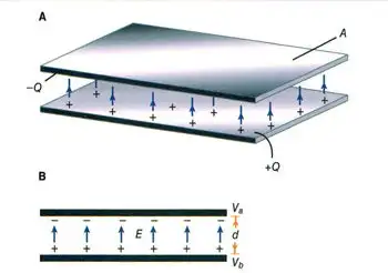
Capacitance is the ability of a capacitor to store electrical charge. A capacitor consists of two conductive plates separated by a dielectric material. The conductive plates are connected to an electrical circuit, and the dielectric material is placed between them to prevent direct contact. When a voltage source is applied to the plates, electrical charge builds up on the surface of the plates. The amount of charge that a capacitor can store is determined by its capacitance, which depends on the size and distance between the plates, as well as the dielectric constant of the material.

The energy storing capability of a capacitor is based on its capacitance. This means that a capacitor with a higher capacitance can store more energy than a capacitor with a lower capacitance. The energy stored in a capacitor is given by the formula:

Energy (Joules) = 0.5 x Capacitance (Farads) x Voltage^2

The ability to store energy is essential for many applications, including filtering, timing, and power conversion. Capacitors are commonly used in DC circuits to smooth out voltage fluctuations and prevent noise. They are also used in AC circuits to filter out high-frequency signals.


What is Capacitance and the SI Unit of Capacitance?

Capacitance is defined as the ratio of the electrical charge stored on a capacitor to the voltage applied to it. The SI unit of capacitance is the Farad (F), which is defined as the amount of capacitance that stores one coulomb of electrical charge when a voltage of one volt is applied. One Farad is a relatively large unit of capacitance, and most capacitors have values that are much smaller. Therefore, capacitors are often measured in microfarads (µF) or picofarads (pF).

The capacitance of a capacitor depends on several factors, including the distance between the plates, the surface area of the plates, and the dielectric constant of the material between the plates. The dielectric constant is a measure of the ability of the material to store electrical energy, and it affects the capacitance of the capacitor. The higher the dielectric constant of the material, the higher the capacitance of the capacitor.


What is the Difference Between Capacitor and Capacitance?

Capacitor and capacitance are related concepts but are not the same thing. Capacitance is the ability of a capacitor to store electrical energy, while a capacitor is an electronic component that stores electrical charge. A capacitor consists of two conductive plates separated by a dielectric material, and it is designed to store electrical charge. Capacitance is a property of a capacitor, and it determines the amount of electrical charge that the capacitor can store. Capacitance is measured in Farads, while the capacitor is measured in units of capacitance, such as microfarads (µF) or picofarads (pF).


What is an Example of Capacitance?

One example of capacitance is a common electronic component known as an electrolytic capacitor. These capacitors are used in a wide range of electronic circuits to store electrical energy, filter out noise, and regulate voltage. They consist of two conductive plates separated by a dielectric material, which is usually an electrolyte. The electrolyte allows for a high capacitance, which means that these capacitors can store a large amount of electrical energy.

Another example of capacitance is the human body. Although the capacitance of the human body is relatively small, it can still store a significant amount of electrical charge. This is why people can sometimes feel a shock when they touch a grounded object, such as a metal doorknob or a handrail. The capacitance of the human body is affected by several factors, including the size and shape of the body, as well as the material and proximity of the objects it comes into contact with.

Related News

Electricity Supply And Demand Balance

Electricity supply covers generation, transmission, distribution, grid infrastructure, voltage regulation, frequency control, power quality, protection, SCADA, and load management to ensure reliable energy delivery to industrial, commercial, and residential loads.


What Is Electricity Supply?

Electricity supply is generation, transmission and distribution of power with set voltage, frequency and reliability.

✅ Involves generation, HV transmission, MV/LV distribution networks

✅ Ensures voltage regulation, frequency control, and power quality

✅ Uses SCADA, protection relays, and load forecasting for reliability


What Is Electricity Supply?

Electricity Supply is a complex balanced system of electric power generation and real time customer demand. Production (supply) and consumption (demand) dictate electricity pricing in the United States and Canada.  For a regional view, the analysis at Electricity Demand in Canada highlights how seasonal peaks and resource availability shape prices.

Where does the term "electricity supply" originate? How does that supply move from one point to another? These are most important questions to ask when you want to understand the electric power industry.

If you're new to the vocabulary, the concise glossary at Electricity Terms can clarify definitions used throughout the industry.

The first thing to know is that electric power is generated in the United States and Canada in power plants which house electrical generators. Then, power is transported (transmission and distriubtution) through the power grid to the customer. This complex network of transmission lines delivers power to industrial, commercial, institutional and residential customers. For a step-by-step overview of system operations, Electricity: How It Works explains generation, transmission, and distribution in practical detail.

In the electricity industry, transmission and distribution wires do the work of transporting power to satisfy electricity demand during real time peak demand. This is the job of the electricity market. The natural gas and fossil fuels industry works in the same way. These lines run from generating station to substations (sometimes over great distances, like in the case of British Columbia and Manitoba where generation is in the far north and the consumption is in the south. This is where the voltage is reduced for local consumption. Substations are usually located close to where the electricity is consumed. 

For background on core power concepts, the primer at Electricity Power connects voltage, current, and load to real-world grid behavior.

The various prices of electricity depends on the electricity supply mix and the energy efficiency of the customer. Electricity energy supply is usually measured in terawatt hours.

The system design is of three-phase alternating current electrical generation and distribution, which was invented by Nikola Tesla in the 19th century. He considered that 60 Hz was the best frequency for alternating current (AC) power generating Electricity Supply. He preferred 240 V, which was claimed to be better for long supply lines. Thomas Edison developed direct current (DC) systems at 110 V and this was claimed to be safer. For more information about the early battles between proponents of AC and DC supply systems see War of Currents. For foundational fundamentals beyond this history, the overview at What Is Electricity clarifies the principles common to both AC and DC systems.

The German company AEG built the first European generating facility to run at 50 Hz, allegedly because the number 60 did not fit into the numerical unit sequence of 1, 2, 5…. At that time, AEG had a virtual monopoly and their standard spread to the rest of the continent. In Britain, differing frequencies (including 25 Hz 40 Hz and DC) proliferated, and the 50 Hz standard was established only after World War II.

To see how frequency standards interact with generation and end-use performance, the explainer at How Electricity Works ties design choices to everyday operation.

Originally much of Europe was 110 V too, just like the Japanese and the US system today. It was deemed necessary to increase the necessary voltage to draw more electrical power with reduced energy loss and voltage drop from the same copper wire diameter.

The choice of utilization voltage is governed more by tradition than by optimization of the distribution system. In theory, a 240 V distribution system will use less conductor material to deliver a given quantity of power. Incandescent lamps for 120 V systems are more efficient and rugged than 240 V lamps, while large heating appliances can use smaller conductors at 240 V for the same output rating. Practically speaking, few household appliances use anything like the full capacity of the outlet to which they are connected. Minimum wire sizes for hand-held or portable equipment is usually restricted by the mechanical strength of the conductors. One may observe that both 240 V system countries and 120 V system countries have extensive penetration of electrical appliances in homes. National electrical codes prescribe wiring methods intended to minimize the risk of electric shock or fire. For household applications, home electricity basics show how these voltage considerations affect outlets, circuits, and safety practices.

Areas using (approximately) 120V allow different combinations of voltage, suitable for use by a variety of classes of electrical equipment.


Related Articles

View more

Thevenin's Theorem

Thevenin’s Theorem simplifies complex linear circuits into a single voltage source and series resistance, making circuit analysis easier for engineers. It helps calculate current, load behavior, and equivalent resistance in practical electrical systems.


What is Thevenin’s Theorem?

Thevenin’s Theorem is a method in circuit analysis that reduces any linear electrical network to an equivalent circuit with a voltage source (Vth) in series with a resistance (Rth).

✅ Simplifies circuit analysis for engineers and students

✅ Calculates load current and voltage with accuracy

✅ Models equivalent resistance for real-world applications

Thevenin’s Theorem allows any linear, two-terminal circuit to be represented by a single voltage source in series with a resistance.

  • Reduces complex circuits to a simple equivalent consisting of a voltage source and a resistor

  • Makes analyzing load response and network behavior straightforward, saving time and effort

  • Widely used for calculating current, voltage, or power across loads in electrical networks

To fully grasp why Thevenin’s Theorem matters, it helps to revisit the principles of basic electricity, where voltage, current, and resistance form the foundation of all circuit analysis.


Understanding Thevenin’s Theorem

Thevenin’s Theorem is a cornerstone of basic electrical engineering and circuit analysis. First introduced by French engineer Léon Charles Thévenin in the late 19th century, the theorem allows engineers and students alike to simplify a complex electrical network to a single voltage source (known as the Thevenin voltage, Vth) in series with a single resistor (known as the Thevenin resistance, Rth). This is particularly useful when analyzing how a circuit will behave when connected to different loads. Concepts such as Ohm’s Law and electrical resistance work in conjunction with Thevenin’s method, ensuring accurate load and network calculations.

Thevenin’s Theorem states that any linear electrical network can be simplified to an equivalent circuit consisting of a single voltage source in series with a resistance. By removing the load resistance, engineers can calculate the equivalent circuit voltage at the terminals, which represents how the circuit will behave when reconnected. This approach replaces multiple components and ideal voltage sources with one simplified model, making circuit analysis more efficient while preserving accuracy in predicting load behavior.


How Thevenin’s Theorem Works

According to Thevenin’s Theorem, no matter how complicated a linear circuit may be, with multiple sources and resistors, it can be replaced by an equivalent Thevenin circuit. This greatly simplifies the process when you’re only interested in the voltage, current, or power delivered to a specific part of the circuit. The steps typically followed when using Thevenin’s Theorem are:

  1. Identify the portion of the circuit for which you want to find the Thevenin equivalent (usually across two terminals where a load is or will be connected).

  2. Remove the load resistor and determine the open-circuit voltage across the terminals. This voltage is the Thevenin voltage (Vth).

  3. Calculate the Thevenin resistance (Rth) by deactivating all independent voltage sources (replace them with short circuits) and current sources (replace them with open circuits), then determining the resistance viewed from the terminals.

  4. Redraw the circuit as a single voltage source Vth in series with resistance Rth, with the load resistor reconnected.


Why Use Thevenin’s Theorem?

There are several reasons why Thevenin’s Theorem is so widely used in both academic and practical electrical engineering:

  • Simplification – Instead of solving a complex network repeatedly each time the load changes, engineers can just reconnect different loads to the Thevenin equivalent, saving time and reducing the potential for error.

  • Insight – By reducing a circuit to its essential characteristics, it’s easier to understand how changes will affect load voltage, current, or power.

  • Foundation for Further Analysis – Thevenin’s Theorem forms the basis for other network analysis techniques, such as Norton's Theorem, and is fundamental to understanding more advanced topics like maximum power transfer.


Example Application

Imagine a scenario where you need to analyze a circuit with multiple resistors and voltage sources connected in series, with a load resistor at the end. Without Thevenin’s Theorem, calculating the voltage across or current through the load each time you change its resistance would require solving complicated sets of equations. Thevenin’s Theorem allows you to do all the hard work once, finding Vth and Rth, and then quickly see how the load responds to different values.

Illustrative Case: A power supply circuit needs to be tested for its response to varying loads. Instead of recalculating the entire network for each load, the Thevenin equivalent makes these calculations swift and efficient. A deeper look at capacitance and inductance shows how energy storage elements influence circuit behavior when simplified through equivalent models.


Limitations and Conditions

While powerful, Thevenin’s Theorem has limitations:

  • It only applies to linear circuits, those with resistors, sources, and linear dependent sources.

  • It cannot directly simplify circuits containing nonlinear elements such as diodes or transistors in their nonlinear regions.

  • The theorem is most useful for “two-terminal” or “port” analysis; it doesn’t help as much with multiple output terminals simultaneously, though extensions exist.


Connections to Broader Electrical Concepts

Thevenin’s Theorem is closely related to other concepts, such as Norton’s Theorem, which prescribes an equivalent current source and parallel resistance. Both theorems are widely applied in real-world scenarios, including power distribution, signal analysis, and the design of electronic circuits. For example, it's relevant when considering how hydro rates impact load distribution in utility networks.

Thevenin’s Theorem is more than just a trick for simplifying homework—it is a core analytical tool that forms the backbone of practical circuit analysis. Whether you are a student learning circuit theory or an engineer designing power systems, understanding and applying Thevenin’s Theorem is essential.  Understanding current flow and the role of a conductor of electricity provides practical insight into why reducing networks to simple equivalents makes engineering analysis more efficient.


Related Articles


View more

Kirchhoff's Law

Kirchhoff's Law, comprising the Current Law (KCL) and Voltage Law (KVL), governs electrical circuits by ensuring charge conservation and energy balance, essential for analyzing current flow, voltage drops, and network behaviour.


What is Kirchhoff's Law?

Kirchhoff's law is an essential principle in the analysis of electrical circuits, enabling a comprehensive understanding of the behaviour of complex circuits.

✅ Defines relationships between currents and voltages in electrical circuits

✅ Ensures conservation of charge (KCL) and energy (KVL) in networks

✅ Essential for analyzing and solving complex circuit problems

It consists of two fundamental rules, Kirchhoff's Current Law (KCL) and Kirchhoff's Voltage Law (KVL), which are intrinsically linked to other electricity laws, such as Ohm's law.  Kirchhoff’s Law works closely with Ohm’s Law Formula to calculate voltage drops, currents, and resistance in electrical networks.

Kirchhoff's Current Law (KCL) - Also known as the first Kirchhoff's law or Kirchhoff's junction rule, KCL states that the sum of the currents entering a junction in a circuit is equal to the sum of the currents leaving the junction. Mathematically, it can be expressed as:

ΣI_in = ΣI_out

KCL is based on the principle of the conservation of charge, asserting that charge can neither be created nor destroyed. In practical terms, KCL means that, at any given point in a circuit, the total current entering must equal the total current leaving, ensuring a continuous flow of electric charge. Understanding Basic Electricity provides the foundation for applying Kirchhoff’s Current Law and Voltage Law to real-world circuit analysis.

Kirchhoff's Voltage Law (KVL) - Also known as the second Kirchhoff's law or Kirchhoff's loop rule, KVL states that the sum of the voltage gains and losses (potential differences) around any closed loop in a circuit is zero. Mathematically, it can be expressed as:
ΣV_rise = ΣV_drop

KVL is based on the principle of the conservation of energy, indicating that energy cannot be created or destroyed but can only be converted from one form to another. In electrical circuits, KVL implies that the total voltage supplied in a loop equals the total voltage drop across all components, ensuring that energy is conserved. Accurate circuit calculations require a clear grasp of Electrical Resistance and how it impacts voltage distribution across components.


Relation to Other Electricity Laws

The most significant connection between Kirchhoff's and other electricity laws is Ohm's law, which defines the relationship between voltage, current, and resistance in an electrical circuit. Ohm's law can be expressed as:

V = IR

When analyzing a circuit using Kirchhoff's laws, Ohm's law is often employed to calculate unknown quantities such as voltage drops, currents, or resistance values. By combining Kirchhoff's laws with Ohm's law, a complete understanding of the behaviour of electrical circuits can be achieved, facilitating efficient design, troubleshooting, and optimization. Applying Kirchhoff’s principles is easier when you understand key Electrical Terms used in engineering and troubleshooting.


History

Gustav Robert Kirchhoff, a German physicist, made significant contributions to understanding electrical circuits by establishing two fundamental laws: Kirchhoff's Voltage Law (KVL) and Kirchhoff's Current Law (KCL). These laws are essential tools for circuit analysis, enabling engineers to design and troubleshoot electrical networks efficiently. In addition to resistance, Capacitance plays a vital role in determining circuit behavior, especially in AC systems.

KVL, also known as the loop rule, states that the algebraic sum of all the voltages around a closed loop equals zero. This principle is derived from the conservation of energy, which ensures that no energy is lost within a closed system. In essence, KVL states that the energy supplied to a circuit is equal to the energy consumed by the components in that circuit. Therefore, when solving problems using KVL, it is essential to consider voltage drops across resistive elements like resistors and voltage rises due to sources like batteries or generators.

On the other hand, KCL, or the junction rule, states that the algebraic sum of currents entering a junction (node) in a circuit is equal to the sum of currents leaving the same junction. This law is a consequence of the conservation of charge, which posits that charge cannot be created or destroyed within an electrical circuit. KCL ensures that the total charge entering and leaving a node remains constant, with the currents (I1, I2, I3, I4, I5) balancing each other. Knowledge of Voltage Drop is essential when using KVL to assess energy losses in electrical circuits.

The significance of these laws in electrical networks lies in their versatility, as they can be applied to a wide range of circuits, from simple series and parallel circuits to more complex electrical networks. Kirchhoff's laws can be employed in conjunction with Ohm's Law, which states that the current through a conductor is proportional to the voltage across it and inversely proportional to its resistance. Using Kirchhoff's and Ohm's Law, engineers can analyze various aspects of a circuit, including voltage drops, current flow, and power distribution.

When analyzing series and parallel circuits, his laws offer valuable insight into the behaviour of electrical components. In series circuits, the current remains constant throughout the entire loop, while the voltage drops across each resistor are proportional to their respective resistances. The voltage across each branch is constant in parallel circuits, but the current is divided among the parallel resistors according to their resistances. By applying KVL and KCL to these configurations, engineers can determine the optimal arrangement of components for a given application.

To illustrate the application of his laws, consider a simple example. Imagine a circuit with a battery, two resistors in series, and a capacitor in parallel with the second resistor. By applying KVL and KCL, we can determine the voltage drop across each resistor, the current flow through each branch, and the voltage across the capacitor, enabling us to analyze the circuit's behaviour under various conditions.

Despite their usefulness, his laws have some limitations and assumptions. For instance, they assume that the components in a circuit are ideal, meaning they have no internal resistance or capacitance. Additionally, they don't account for the effects of electromagnetic fields or the finite speed of signal propagation in AC circuits. However, these limitations are often negligible in many practical applications, as they only marginally impact circuit performance. For a deeper historical context, explore the History of Electricity and the contributions of Gustav Kirchhoff to modern circuit theory.


Related Articles


View more

Windmills For Electricity Explained

Windmills for electricity use wind energy to generate clean, renewable power. These wind turbines convert kinetic energy into electrical energy, reducing carbon emissions and dependence on fossil fuels. 


What are Windmills for Electricity?

Windmills for electricity are modern devices that transform kinetic wind energy into electrical power.

✅ Harness renewable energy for clean power

✅ Reduce carbon footprint and dependence on fossil fuels

✅ Support sustainable power generation worldwide

Windmills for electricity are part of a broader shift toward renewable energy, providing clean alternatives to fossil fuels for homes, businesses, and utilities.


History of Windmills

Windmills for electricity - Mankind has been harnessing the wind's energy for many years. From Holland to traditional farms around the world, windmills were used in the past for pumping water through primitive irrigation systems or to grind grain. Then, the wind turned large "sails" that were connected by a long vertical shaft, which was attached to a grinding machine or a wheel that turned and drew water from a well. Today's turbines harness the energy of the wind to turn large metal blades, which in turn spin a generator that produces electric power. Alongside wind, other renewable energy sources like solar, biomass, and tidal energy are shaping a diversified and sustainable energy future.

From the mid-1970s to the mid-1980s, the United States government collaborated with industry to advance windmill technology for power generation and enable the development of large commercial wind turbines. NASA led this effort at the Lewis Research Center in Cleveland, Ohio, and it was an extraordinarily successful government research and development activity.


National Science Foundation

With funding from the National Science Foundation and later the Department of Energy (DOE), a total of 13 experimental wind turbines were put into operation, including four major wind turbine designs. This research and development program pioneered many of the multi-megawatt turbine technologies in use today, including steel tube towers, variable-speed generators, composite blade materials, partial-span pitch control, as well as aerodynamic, structural, and acoustic engineering design capabilities. The large Windmills For Electricity developed under this effort set several world records for diameter and power output. The Mod-2 wind turbine cluster produced a total of 7.5 megawatts of power in 1981. Government incentives, such as alternative energy tax credits, have played a major role in expanding wind power adoption across North America.


Wind Turbine Technology

In 1987, the Mod-5B was the largest single wind turbine operating in the world with a rotor diameter of nearly 100 meters and a rated power of 3.2 megawatts. It demonstrated an availability of 95 percent, an unparalleled level for a new first-unit wind turbine. The Mod-5B featured the first large-scale variable-speed drive train and a sectioned, two-blade rotor, which enabled easy transport of the blades.

Later, in the 1980s, California provided tax rebates for ecologically harmless wind turbines. These rebates helped fund the first major deployment of wind power for the utility grid. These turbines gathered in large wind parks such as at Altamont Pass, would be considered small and uneconomical by modern wind power development standards.

In the 1990s, as aesthetics and durability became more important, turbines were placed atop steel or reinforced concrete towers. Small generators are connected to the ground tower, and then the tower is raised into position. Larger generators are hoisted into position atop the tower, and a ladder or staircase is located inside the tower to allow technicians to reach and maintain the generator.

Originally, wind turbines were built right next to where their power was needed. With the availability of long-distance electric power transmission, wind generators are now often on wind farms in windy locations, and huge ones are being built offshore, sometimes transmitting power back to land using high-voltage submarine cable. Since wind turbines are a renewable means of generating power, they are being widely deployed, but their cost is often subsidized by taxpayers, either directly or through renewable energy credits. Much depends on the cost of alternative energy sources. The cost of wind generators per unit of power has been decreasing by about 4% per year.


Modern Wind Turbines

The most modern generations of Windmills for electricity are more properly called wind turbines, or wind generators, and are primarily used to generate electric power. Modern windmills are designed to harness the energy of the wind and convert it into electric energy. The largest wind turbines can generate up to 6 MW of power (for comparison, a modern fossil fuel power plant generates between 500 and 1,300 MW). Many large-scale renewable energy projects now combine wind farms with solar and storage systems, ensuring reliable, clean power for communities worldwide.

Small wind turbines can generate as little as a few kilowatts, while larger models produce up to 100 kilowatts or more, depending on design and location. These devices capture moving air, and as wind turbines operate, the kinetic energy generated can be used directly or sent into the electrical grid. On a utility scale, wind farms combine many large turbines to deliver massive amounts of energy, powering thousands of homes and businesses. This range of applications, from residential to industrial, demonstrates the versatility of wind technology in meeting diverse energy needs.


Related Articles


View more

Electrical Resistance Definition Explained

Electrical resistance definition explains how materials oppose current flow in circuits, measured in ohms, linked to voltage, resistivity, conductor geometry, temperature, and impedance, governed by Ohm's law and SI units in electronics.


What Is Electrical Resistance Definition?

It is the measure of how a material opposes electric current, equal to voltage divided by current and measured in ohms.

✅ Measured in ohms; per Ohm's law, resistance R equals voltage V over current I.

✅ Depends on material resistivity, length, cross-sectional area, and temperature.

✅ Key in circuit analysis, power dissipation, signal integrity, and safety.


Electrical Resistance Definition: ER occurs in an electrical circuit when current-carrying charged particles collide with fixed particles that make up the structure of the conductors. Resistance is measured in ohm. Resistance is the ohm w. Resistance occurs in every part of a circuit, including wires and especially power transmission lines. For a concise overview, see this introduction to electrical resistance to reinforce key definitions.

Dissipation of electric energy in the form of heat affects the amount of driving voltage required to produce a given current through the circuit. In fact, volts are mesured across a circuit divided by the current I (amperes) through that circuit defines quantitatively the amount of electrical resistance R. The ohm is the common unit of electrical resistance, equivalent to one volt per ampere and represented by the capital Greek letter omega, Ω. The electrical resistance of a wire is directly proportional to its length and inversely proportional to its cross-sectional area. Resistance also depends on the material of the conductor. For instance, the resistance of a conductor generally increases with increasing temperature the resistivity. This is why some conductors have almost zero resistance when cooled to extremely low temperatures, as is the case with superconductors, because of the relative resistivity of metals. There is a temperature coefficient of resistivity. If you need a refresher on potential difference and its role in circuits, review this explanation of voltage to connect the concepts.

Alternating-current resistors for current measurement require further design consideration. For example, if the resistor is to be used for current-transformer calibration, its ac resistance must be identical with its dc resistance within 1/100th% or better, and the applied voltage difference between its voltage terminals must be in phase with the current through it within a few tenths of a minute. Thin strips or tubes of resistance material are used to limit eddy currents and minimize "skin" effect, the current circuit must be arranged to have small self-inductance, and the leads from the voltage taps to the potential terminals should be arranged so that, as nearly as possible, the mutual inductance between the voltage and current circuits opposes and cancels the effect of the self-inductance of the current circuit. In (a) a metal strip has been folded into a very narrow U; in (b) the current circuit consists of coaxial tubes soldered together at one end to terminal blocks at the other end; in (c) a straight tube is used as the current circuit, and the potential leads are snugly fitting coaxial tubes soldered to the resistor tube at the desired separation and terminating at the center. These design choices are also easier to contextualize by comparing common types of resistors used for precise AC measurements.

Electrical Resistance coils consist of insulated resistance copper wire wound on a bobbin or winding form, hard-soldered at the ends to copper terminal wires. Metal tubes are widely used as winding form for dc resistors because they dissipate heat more readily than insulating bobbins, but if the resistor is to be used in ac measurements, a ceramic winding form is greatly to be preferred because it contributes less to the phase-defect angle of the resistor. The resistance wire ordinarily is folded into a narrow loop and wound bifilar onto the form to minimize inductance. This construction results in considerable associated capacitance of high-resistance coils, for which the wire is quite long, and an alternative construction is to wind the coil inductively on a thin mica or plastic card. The capacitive effect is greatly reduced, and the inductance is still quite small if the card is thin. When specifying coil assemblies, it helps to recall the standardized unit of electrical resistance so ratings and tolerances are interpreted consistently.

Resistors in which the wire forms the warp of a woven ribbon have lower time constants than either the simple bifilar- or card-wound types. Manganin is the resistance material most generally employed, but Evanohm and similar alloys are beginning to be extensively used for very high resistance coils. Enamel or silk is used to insulate the wire, and the finished coil is ordinarily coated with shellac or varnish to protect the wire from the atmosphere. Such coatings do not completely exclude moisture, and dimensional changes of insulation with humidity will result in small resistance changes, particularly in high resistances where fine wire is used. Material behavior, moisture effects, and long term stability are discussed further in this broader overview of electrical resistance for additional context.

Electrical Resistance boxes usually have two to four decades of resistance so that with reasonable precision they cover a considerable range of resistance, adjustable in small steps. For convenience of connection, terminals of the individual resistors are brought to copper blocks or studs, which are connected into the circuit by means of plugs or of dial switches using rotary laminated brushes; clean, well-fitted plugs probably have lower resistance than dial switches but are much less convenient to use. The residual inductance of decade groups of coils due to switch wiring, and the capacitance of connected but inactive coils, will probably exceed the residuals of the coils themselves, and it is to be expected that the time constant of an assembly of coils in a decade box will be considerably greater than that of the individual coils. Understanding how series and parallel combinations set the equivalent resistance will inform how decade boxes are deployed in complex networks.

Measurement of resistance is accomplished by a variety of methods, depending on the magnitude of the resistor and the accuracy required. Over the range from a few ohms to a megohm or more, an ohmmeter may be used for an accuracy of a few percent. A simple ohmmeter may consist of a milliammeter, dry cell, and resistor in a series circuit, the instrument scale being marked in resistance units, if you obey ohm law. For a better value, the voltage drop is measured across the resistor for a measured or known current through it. Here, accuracy is limited by the instrument scales unless a potentiometer is used for the current and voltage measurements. The approach is also taken in the wide variety of digital multimeters now in common use. Their manufacturers' specifications indicate a range of accuracies from a few percent to 10 ppm (0.001%) or better from the simplest to the most precise meters. Bridge methods can have the highest accuracy, both because they are null methods in which two or more ratios can be brought to equality and because the measurements can be made by comparison with accurately known standards. For two-terminal resistors, a Wheatstone bridge can be used; for four-terminal measurements, a Kelvin bridge or a current comparator bridge can be used. Bridges for either two- or four-terminal measurements also may be based on resistive dividers. Because of their extremely high input impedance, digital voltmeters that be used with standard resistors in unbalanced bridge circuits of high accuracy. For quick reference during test planning, the fundamental resistance formula clarifies how R, V, and I are related under Ohm law.

Digital multi meters are frequently used to make low-power measurements of resistors in the range between a few ohms and a hundred megohms or so. Resolution of such instruments varies from 1% of full scale to a part per million of full scale. These meters generally use a constant-current source with a known current controlled by comparing the voltage drop on an internal "standard" resistor to the EMF produced by a Zener diode. The current is set at such a level as to make the meter direct-reading in terms of the displayed voltage; that is, the number displayed by the meter reflects the voltage drop across the resistor, but the decimal point is moved and the scale descriptor is displayed as appropriate. Multimeters typically use three or more fixed currents and several voltage ranges to produce seven or more decade ranges with the full-scale reading from 1.4 to 3.9 times the range. For example, on the 1000-0 range, full scale may be 3,999.999 Q. Power dissipated in the measured resistor generally does not exceed 30 mW and reaches that level only in the lowest ranges where resistors are usually designed to handle many times that power. The most accurate multimeters have a resolution of 1 to 10 ppm of range on all ranges above the 10-0 range. Their sensitivity, linearity, and short-term stability make it possible to compare nominally equal resistors by substitution with an uncertainty 2 to 3 times the least count of the meter. This permits their use in making very accurate measurements, up to 10 ppm, or resistors whose values are close to those of standards at hand. Many less expensive multimeters have only two leads or terminals to use to make measurements. In those cases, the leads from the meter to the resistor to be measured become part of the measured


Related Articles

View more

Prospective Fault Current Meaning Explained

Prospective fault current (PFC) is the highest electric current that can flow in a system during a short circuit. It helps determine equipment ratings, breaker capacity, and safety measures in electrical installations to prevent overheating, fire, or component failure.


What is the Meaning of Prospective Fault Current?

Prospective fault current refers to the maximum current expected during a short circuit at any point in an electrical system.

✅ Helps size circuit breakers and fuses for safe disconnection

✅ Ensures compliance with installation and safety codes

✅ Prevents equipment damage from excessive short-circuit current

Prospective fault current (PFC) is a key factor in the safety and design of electrical systems. It represents the maximum current that could flow in the event of a fault, such as a short circuit. Understanding PFC is essential for selecting protective devices that can handle fault conditions safely. This article explores what PFC is, how it is measured, and its importance for electrical installations, while addressing key questions. Understanding electrical short circuits is key to calculating prospective fault current and ensuring system safety.

When measuring prospective short circuit current in an electrical system, it’s essential to perform tests between L1 N CPC and L2 N CPC to assess the fault current across different phases and protective conductors. These measurements help identify the maximum prospective fault current present in the system, especially at points involving live conductors. Whether taking note of a single-phase supply or between line conductors on a three-phase supply, proper testing protocols must be followed. Technicians should always use insulated test leads rated for the expected voltage and current levels, and please refer to the test meter manufacturer’s instruction for safe and accurate operation. Reliable results ensure that the protective devices can safely interrupt fault conditions, preventing system damage and ensuring compliance with fault current protection standards.


Frequently Asked Questions

Why is it Important?

Prospective fault current refers to the maximum current that could pass through a system during a fault. The PFC helps determine the breaking capacity of fuses and circuit breakers, ensuring these protective devices can handle high currents safely. This is vital for protecting the electrical installation and those working near it.

Understanding PFC is critical for ensuring increased safety for employees and third parties. Protective devices must be selected to handle PFC; otherwise, they may fail to operate correctly, leading to severe consequences, such as fires or injuries. To fully grasp how PFC affects energy flow, it’s useful to review the concept of electrical resistance in a circuit.


How is Prospective Fault Current Measured or Calculated?

PFC can be measured or calculated using tools such as a multifunction tester, often during fault current testing. The instrument uses a single-phase supply or between line conductors on a three-phase supply to measure the maximum potential current at various points in the installation. Testing often involves checking currents between L1 N CPC, L2 N CPC, and L3 N CPC, which measure current between the lines to neutral in a three-phase system.

When performing these tests, technicians should follow regulation 612.11 of a single-phase supply or between line conductors on a three-phase supply, ensuring that simple and circuit protective conductors are all connected correctly. Accurate testing must also account for maximum current flow. Live testing requires extreme caution, and it is important to refer to the test meter manufacturer’s instructions to ensure proper usage and safety. In three-phase systems, 3-phase electricity significantly impacts how fault current behaves during a short circuit.


What is the difference between PFC and Short-Circuit Current?

Though often confused, prospective fault current and short-circuit current are distinct. Prospective fault current is the theoretical maximum current that could flow in a fault, used to predict the worst-case scenario for selecting protective devices. Short-circuit current refers to the actual current that flows during a fault, which depends on real-time conditions such as circuit impedance. Prospective fault current is one of the many concepts that form the foundation of electricity fundamentals.


How Does Prospective Fault Current Impact the Selection of Protective Devices?

The calculation of PFC plays a critical role in selecting the correct protective devices. Circuit breakers and fuses must have a breaking capacity that matches or exceeds the prospective fault current in the system. If the PFC exceeds the breaking capacity, the protective device may fail, leading to dangerous electrical hazards.

For instance, fault current testing using a multifunction tester between phases and neutral (L1, L2, L3) ensures that protective devices are rated to handle the highest potential fault current in the system. Proper circuit protection ensures that the system can interrupt faults safely, minimizing the risks to workers and equipment.


What Standards and Regulations Govern Prospective Fault Current Calculations?

Various standards, such as IEC 60909, govern how PFC is calculated and how protective devices are selected. These regulations ensure that electrical systems are designed to handle maximum fault conditions safely. Regulation 612.11 further specifies how live testing should be conducted using proper equipment and safety protocols.

It is essential to test PFC at relevant points in the system and follow testing standards to ensure compliance and safety. Devices selected based on PFC calculations help ensure that electrical systems can withstand faults and maintain reliable operation.

Prospective fault current is a crucial element in the safety and reliability of electrical installations. By calculating PFC, engineers can select protective devices that ensure safe operation in the event of a fault. Testing for fault currents at different points in the system and adhering to regulations are essential steps in preventing hazardous conditions.

By choosing protective devices with the appropriate breaking capacity and following safe testing practices, electrical installations can handle fault conditions and protect both workers and equipment from harm. Selecting protective devices that match the PFC is essential for reliable electric power systems design.


Related Articles


View more

Sign Up for Electricity Forum’s Newsletter

Stay informed with our FREE Newsletter — get the latest news, breakthrough technologies, and expert insights, delivered straight to your inbox.

Electricity Today T&D Magazine Subscribe for FREE

Stay informed with the latest T&D policies and technologies.
  • Timely insights from industry experts
  • Practical solutions T&D engineers
  • Free access to every issue

Download the 2025 Electrical Training Catalog

Explore 50+ live, expert-led electrical training courses –

  • Interactive
  • Flexible
  • CEU-cerified